Excel guide · PivotTable
How to create a pivot table in Excel
A pivot table (Excel calls it a PivotTable) totals a long sales or expense list by region, month or product in a few clicks. Below is how to create one in Excel step by step; then we show how to build the same table in Nexell with a single sentence.
Free account · no card · 30 credits a month · Not ready to sign up? Paste some text and try it
Step by step
How to create a pivot table in Excel
-
1
Prepare the list
Give every column a one-row header and leave no blank rows or merged cells in the list. Convert the list with Insert > Table: rows you add later join the pivot table when you refresh it.
-
2
Insert the PivotTable
Select a cell in the list and click PivotTable on the Insert tab. Check the range Excel picked, choose New Worksheet and click OK.
-
3
Drag the fields
In the PivotTable Fields pane drop Region into Rows, Category into Columns and Amount into Values. A number field is summed automatically.
-
4
Group and refresh
To total dates by month, right-click a date in the pivot table, choose Group and select Months. A pivot table does not update when the source list changes: right-click it and choose Refresh.
Example
The same pivot table in Nexell: two sentences
We pasted a quarter of sales into the tool and typed two requests.
1Pasted list
2In Nexell
- Text turned into a table: 5 columns, 12 rows. Dates came in as real dates and amounts as numbers.
- format as a tableData will be formatted as an Excel table, filterable and banded
- pivot table: region in rows, category in columns, sum of amountPivot table: Region in rows, Category in columns · Sum of Amount, added as a native PivotTable on its own sheet
The pivot table does not change the list; it is added to the file as a separate sheet.
3In Excel
85820| A | B | C | D | |
|---|---|---|---|---|
| 1 | Sum of Amount by Region × Category | |||
| 2 | ||||
| 3 | Sum of Amount | Category | ||
| 4 | Region | Furniture | Stationery | Grand Total |
| 5 | Central | 23,950.00 | 4,130.00 | 28,080.00 |
| 6 | East | 20,700.00 | 6,440.00 | 27,140.00 |
| 7 | West | 20,600.00 | 10,000.00 | 30,600.00 |
| 8 | Grand Total | 65,250.00 | 20,570.00 | 85,820.00 |
This is Excel's own PivotTable: you can keep changing its fields in the PivotTable Fields pane. Its source is the table on the Data sheet; add rows to the table, right-click the pivot table and choose Refresh, and the new rows are totaled too. Cost: 3 credits (the conversion plus two requests); downloading was free.
Illustrative example with made-up figures; the layout shown is what Nexell writes into the downloaded file.
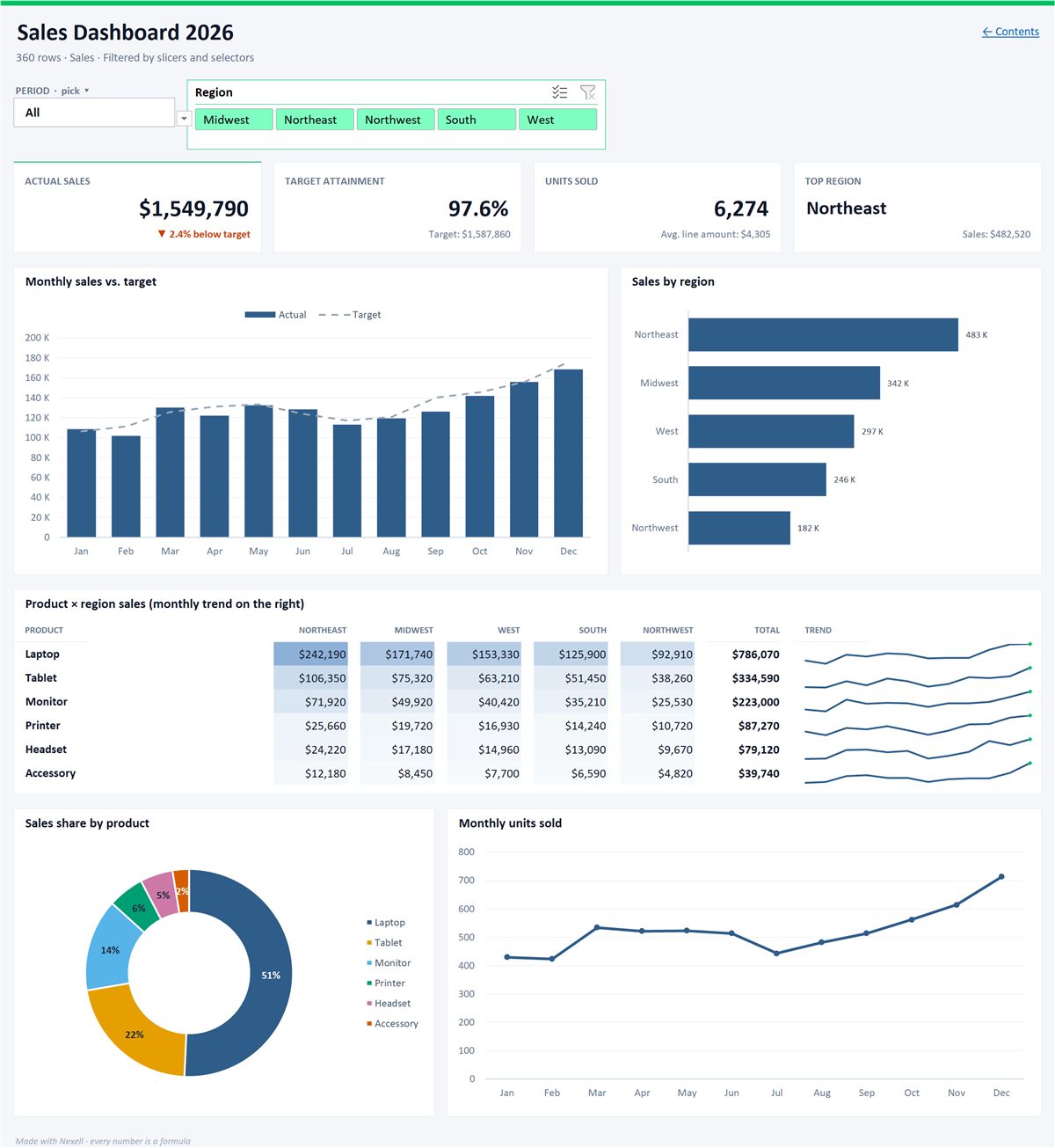
Sales dashboard in Excel
KPI cards, charts and a region slicer. Every number is a real Excel formula.
Why Nexell
What Nexell does differently
A real PivotTable
The pivot table goes into the file as Excel's own refreshable PivotTable, not as fixed numbers, so you keep changing its fields in Excel.
Pick fields by sentence
Write “pivot table: region in rows, category in columns”. The preview says which field goes to rows and which to values.
Starts from a messy list
A PDF, CSV or email list is turned into a clean table first, so amounts become numbers you can total.
Limits
What to know before you start
- Dates are not grouped by month in a short list. With more than 31 different days in the date column, dates are grouped by year and month; in a shorter list each date becomes its own column. In that case right-click a date in Excel and choose Group > Months.
- If you do not say “pivot table”, you get a cross-tab. “Region in rows, month in columns” turns the list into a cross-tab with totals; it holds fixed values and does not refresh. For a refreshable PivotTable, say “pivot table” or “pivot” in the sentence.
- Privacy. Personal data in text is masked before it is sent to the AI service (what is sent).
FAQ
Excel pivot tables: common questions
What is a pivot table?
It is an Excel tool that groups the records in a list by the fields you choose and sums, counts or averages them. The source list does not change; the pivot table sits in a separate area and is recalculated from the source when you refresh it.
How do I update a pivot table in Excel?
Right-click the pivot table and choose Refresh; to refresh every pivot table in the workbook use Refresh All on the Data tab. If the source is an Excel table, new rows are included; if it is a fixed range, widen it with Change Data Source on the PivotTable Analyze tab.
How do I filter a pivot table?
Drag a field into the Filters box of the PivotTable Fields pane, or click the drop-down arrow beside the row or column headings. For button-style filtering, choose Insert Slicer on the PivotTable Analyze tab.
Can I refresh the pivot table Nexell builds in Excel?
Yes. When your sentence says “pivot table” or “pivot”, the file gets Excel's own PivotTable on a separate sheet, with the Data sheet as its source. Change the values, right-click and choose Refresh, and the pivot table is recalculated.
Related
More Excel jobs you can do by typing
- Match two lists without VLOOKUPCompare two lists by a shared code, by typing.
- Conditional formattingColor the rows that cross a threshold, add data bars.
- Excel formula generatorType what to calculate and let Nexell build the formula.
- VAT calculation in ExcelSplit a gross amount into net and VAT with live formulas.
Build the pivot table with one sentence.
Create a free account, bring your data and type what you need.
Try it free